Gilbert Strang's 18.06 Linear Algebra course at MIT is widely considered the best linear algebra course ever recorded. Strang has taught it for decades, and the video lectures on MIT OpenCourseWare have been watched hundreds of millions of times. The course is technically accessible — Strang assumes only basic calculus — but conceptually dense. Two hours of Strang is a lot to absorb in one sitting.
These MIT linear algebra notes cover the full 18.06 curriculum: from the geometry of vectors through matrix factorizations, determinants, eigenvalues, and the singular value decomposition. They are written for students who have watched (or are about to watch) the lectures and want a structured reference to consolidate what they learned.
The official course is available at ocw.mit.edu. These notes are a companion to those lectures.
Lecture 1–2: The Geometry of Linear Equations
Strang opens with a question: what does it mean to solve a system of linear equations? He presents two ways to look at it.
Row picture: Each equation defines a line (in 2D), a plane (in 3D), or a hyperplane (in higher dimensions). The solution is the point where all of them intersect.
Column picture: The same system written as a linear combination of column vectors. Can the vector b be expressed as a combination of the columns of A? This viewpoint — "column space" thinking — turns out to be far more powerful for understanding what linear algebra is really about.
For the system:
2x - y = 0
-x + 2y = 3
Row picture: two lines meeting at a point. Column picture: x * [2, -1] + y * [-1, 2] = [0, 3]. Can we find scalars x and y to produce this combination? Yes: x=1, y=2.
Why the column picture matters: When you extend to n equations in n unknowns, drawing rows (hyperplanes) in high-dimensional space is not intuitive. Column combinations — "does this vector lie in the span of these columns?" — generalizes naturally. Strang emphasizes this repeatedly. Most textbooks lead with the row picture; Strang's insight is that the column picture builds better intuition for the rest of the course.
Matrix-vector multiplication as column combinations:
Ax = b means x₁*(col 1 of A) + x₂*(col 2 of A) + ... = b
This interpretation — Ax is a linear combination of A's columns with weights from x — is the foundation for understanding column space, null space, and everything that follows.
Lectures 3–8: Elimination, Factorization, and Inverses
Gaussian elimination is the algorithmic heart of linear algebra. Starting from an augmented matrix [A | b], systematically eliminate unknowns using row operations until the system is in upper triangular form, then back-substitute.
Pivots: The first nonzero element used in each elimination step. For elimination to succeed, every pivot must be nonzero. If a zero appears in the pivot position, swap rows (partial pivoting). If no swap is possible, the matrix is singular.
LU Factorization:
Every step of Gaussian elimination can be represented as multiplying by an elementary matrix. The product of all these elementary matrices gives us L (lower triangular), and the result of elimination gives us U (upper triangular). So:
A = LU
This factorization is enormously useful. To solve Ax = b for multiple right-hand sides, factor A = LU once (O(n³)), then solve Ly = b and Ux = y for each b (O(n²) each). LU factorization with partial pivoting — PA = LU — is what numpy.linalg.solve uses internally.
Inverse matrices:
A matrix A is invertible (nonsingular) if there exists A⁻¹ such that A⁻¹A = AA⁻¹ = I. Computing A⁻¹ via Gauss-Jordan elimination augments [A | I] and row-reduces to [I | A⁻¹].
Key facts Strang emphasizes:
(AB)⁻¹ = B⁻¹A⁻¹— the order reverses- A matrix is invertible iff its determinant is nonzero
- A matrix is invertible iff elimination produces no zero pivots
- A matrix is invertible iff its null space contains only the zero vector
Transpose:
(A^T)ᵢⱼ = Aⱼᵢ. Transposing swaps rows and columns. Key properties: (AB)^T = B^T A^T, (A⁻¹)^T = (A^T)⁻¹. A symmetric matrix satisfies A^T = A — eigenvalue theory is especially clean for symmetric matrices.
Lectures 9–14: Vector Spaces, Null Space, and the Four Fundamental Subspaces
This is where 18.06 becomes abstract. Strang introduces the four fundamental subspaces of a matrix A (m×n):
- Column space C(A) — all linear combinations of A's columns. Subspace of ℝᵐ.
- Null space N(A) — all vectors x such that Ax = 0. Subspace of ℝⁿ.
- Row space C(A^T) — all linear combinations of A's rows. Subspace of ℝⁿ.
- Left null space N(A^T) — all vectors y such that A^Ty = 0. Subspace of ℝᵐ.
The fundamental theorem of linear algebra (Part 1):
dim(C(A)) = dim(C(A^T)) = r  (the rank of A)
dim(N(A)) = n - r
dim(N(A^T)) = m - r
The rank r is the number of pivots from elimination. All four subspaces are defined by r, n, and m.
What is a subspace?
A subspace of ℝⁿ must satisfy three conditions: (1) contains the zero vector, (2) closed under addition (sum of two vectors in the space is also in the space), (3) closed under scalar multiplication. A plane through the origin in ℝ³ is a subspace. A plane not through the origin is not (it fails condition 1).
Basis and dimension:
A basis for a subspace is a set of linearly independent vectors that span the subspace. The number of vectors in any basis is the dimension. The basis is not unique; the dimension is.
Finding the null space: Row-reduce A to reduced row echelon form (RREF). Identify free variables (columns without pivots). For each free variable, set it to 1 and others to 0, then solve for pivot variables. The resulting vectors are the null space basis — called special solutions.
Rank and the solvability of Ax = b:
The system Ax = b is solvable iff b is in the column space of A. If A is m×n with rank r:
- If r = m: full row rank, Ax = b is solvable for every b (no zero rows in RREF of A)
- If r = n: full column rank, solutions are unique when they exist (no free variables)
- If r = m = n: A is square and invertible, unique solution for every b
Lectures 15–20: Orthogonality, Projections, and Least Squares
Orthogonality:
Vectors x and y are orthogonal if x^T y = 0. Two subspaces are orthogonal if every vector in one is orthogonal to every vector in the other.
Fundamental theorem of linear algebra (Part 2): The row space and null space are orthogonal complements in ℝⁿ. The column space and left null space are orthogonal complements in ℝᵐ. This is Strang's central geometric insight: the four subspaces come in two orthogonal pairs.
Projection:
The projection of vector b onto the line through vector a is:
p = (a^T b / a^T a) * a
More generally, projecting b onto the column space of matrix A:
p = A(A^T A)⁻¹ A^T b
The projection matrix is P = A(A^T A)⁻¹ A^T. Key properties: P² = P (projecting twice gives the same result), P^T = P (symmetric).
Least squares:
When Ax = b has no exact solution (b not in C(A)), the best approximate solution minimizes ‖Ax - b‖². This is least squares. The solution satisfies the normal equations:
A^T A x̂ = A^T b
Least squares is everywhere: linear regression in statistics, curve fitting in engineering, neural network training (in a linearized sense). Understanding the geometry — the projection interpretation — makes the formula intuitive rather than magical. If you're heading toward machine learning, this is foundational. The Coursera deep learning specialization notes build on exactly this.
Gram-Schmidt and QR factorization:
Gram-Schmidt orthogonalization converts any basis into an orthonormal basis. The process generates matrices Q (orthonormal columns) and R (upper triangular) such that A = QR. With orthonormal columns, projections simplify: P = QQ^T, and the normal equations become Q^T Qx̂ = Q^T b, which simplifies to x̂ = Q^T b.
Lectures 21–26: Determinants and Eigenvalues
Determinants:
The determinant of a square matrix encodes whether it is invertible (det ≠ 0) and what happens to volume under the linear transformation. Key properties:
- det(I) = 1
- Swapping rows flips the sign
- Multiplying a row by c multiplies the determinant by c
- det(AB) = det(A) · det(B)
- det(A^T) = det(A)
- det(A⁻¹) = 1/det(A)
The cofactor expansion formula and the rule of Sarrus (for 3×3) are computation methods, not definitions. The three properties above are the definition.
Eigenvalues and eigenvectors:
Vector x is an eigenvector of A with eigenvalue λ if:
Ax = λx
A does not rotate x — it only stretches (or flips) it. To find eigenvalues, solve the characteristic equation:
det(A - λI) = 0
This is a degree-n polynomial in λ. The n roots (counting multiplicity, possibly complex) are the eigenvalues.
Why eigenvalues matter:
They control everything about what happens to a vector under repeated application of A. The sequence x, Ax, A²x, ... converges if all |λᵢ| < 1. It grows if any |λᵢ| > 1. This is the foundation of stability analysis in differential equations, PageRank, Markov chains, and recurrent neural networks.
Diagonalization:
If A has n linearly independent eigenvectors (columns of matrix S), then:
A = SΛS⁻¹
where Λ is a diagonal matrix of eigenvalues. Powers become easy: Aᵏ = SΛᵏS⁻¹, and Λᵏ is just the diagonal matrix with λᵢᵏ entries.
Symmetric matrices (Strang's favorite):
Real symmetric matrices (A^T = A) have: all real eigenvalues, orthogonal eigenvectors. This means S = Q (orthogonal matrix), giving the spectral decomposition:
A = QΛQ^T = λ₁q₁q₁^T + λ₂q₂q₂^T + ... + λₙqₙqₙ^T
Every symmetric matrix is a sum of rank-one projections, weighted by eigenvalues. This decomposition underpins principal component analysis (PCA).
Lectures 27–34: Positive Definite Matrices, SVD, and Linear Transformations
Positive definite matrices:
A symmetric matrix A is positive definite if x^T Ax > 0 for all nonzero x. Equivalent conditions: all eigenvalues positive, all pivots positive, all leading determinants positive. Positive definite matrices are the symmetric analogue of positive numbers — they have square roots, their Cholesky factorization A = R^T R exists, and they are used to define inner products.
The Singular Value Decomposition (SVD):
The SVD is the climax of 18.06. Every m×n matrix A (not just square, not just symmetric) has the factorization:
A = UΣV^T
Where:
- U is m×m orthogonal (columns are left singular vectors)
- Σ is m×n diagonal (singular values σ₁ ≥ σ₂ ≥ ... ≥ 0 on diagonal)
- V^T is n×n orthogonal (columns of V are right singular vectors)
What SVD means geometrically: Every linear transformation is a rotation (V^T), followed by a scaling (Σ), followed by another rotation (U). The singular values measure how much stretching happens in each direction.
Applications of SVD:
- Low-rank approximation: Keep only the top k singular values and vectors. The resulting rank-k matrix is the closest rank-k matrix to A in the Frobenius norm. This is image compression, noise reduction, and the mathematical foundation of recommendation systems.
- PCA: The principal components are the columns of V (right singular vectors of the centered data matrix). The variance explained by each component is proportional to the square of the singular value.
- Pseudoinverse: A⁺ = VΣ⁺U^T where Σ⁺ inverts the nonzero singular values. The pseudoinverse gives the minimum-norm least-squares solution to Ax = b.
- Condition number: σ_max / σ_min measures how sensitive the solution x is to perturbations in b. Large condition number → numerically unstable system.
If you are going deeper into machine learning or data science, SVD is not optional background material — it is central. The Andrew Ng ML course notes and Stanford CS230 deep learning notes both assume you understand matrix decompositions.
Is Gilbert Strang's 18.06 the Right Course for You — And What Prerequisites Do You Actually Need?
18.06 is the right choice if you want to understand linear algebra at the level that makes everything else make sense. If you have taken a linear algebra course that felt like "matrix operations without explanations," Strang's geometric and intuitive approach will reframe everything.
It is demanding. Strang moves quickly, assumes mathematical maturity, and does not repeat himself. Students who get the most from 18.06 typically:
- Have a calculus background (even basic calculus)
- Are comfortable with abstract definitions (subspace, basis, dimension)
- Watch lectures twice: once for the story, once for the details
- Work through the problem sets from the OCW materials
The course pairs naturally with statistics and probability for data science, or with multivariable calculus. If you want to understand the mathematics of neural networks at depth, 18.06 is a prerequisite. For those connections, see learn calculus from YouTube and learn statistics from YouTube.
How to Take Notes on Strang's Lectures — What Actually Sticks?
Strang's lectures are heavy with notation and geometry. The key is to capture both: write down the formula, but also write a one-sentence description of what it means geometrically. If you can only remember the formula and not the geometry, you will not be able to apply it in novel situations.
A practical workflow: watch the lecture, then immediately paste the YouTube URL into a note-taking tool to get an AI-generated outline. Use that outline to fill in your own understanding — anywhere the outline says something you cannot explain in plain words is a gap to revisit.
For the broader strategy of extracting structured notes from any math lecture, see the YouTube to notes complete guide.
Linear algebra is the language of machine learning, statistics, computer graphics, and quantum mechanics. Strang's 18.06 is the most efficient path to actually understanding it rather than just computing with it.
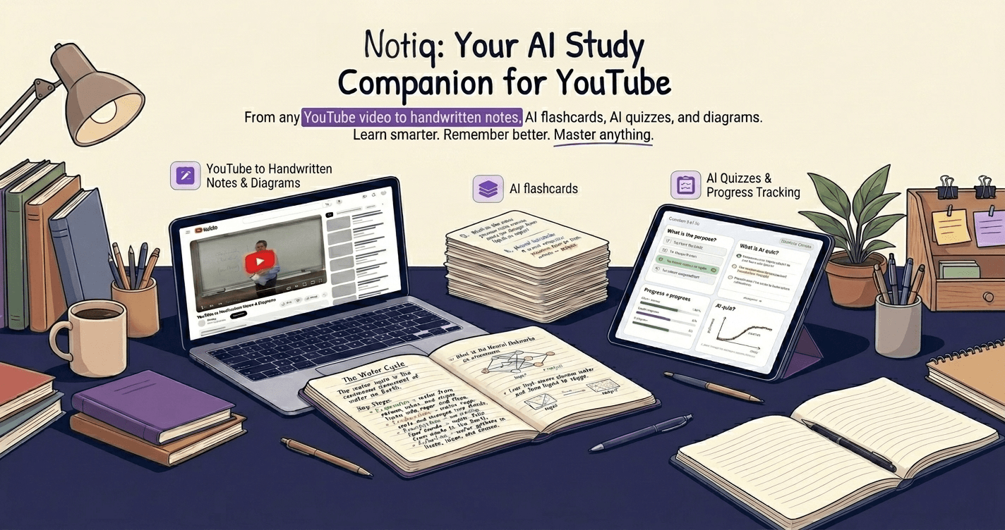
Ready to convert any 18.06 lecture into structured notes and flashcards? Try Notiq free at notiq.study — paste the YouTube URL and get a complete study guide automatically.